HTML Stuff

class: center, middle, inverse, title-slide

# HTML Stuff
## Fonts, Dashboards, Websites & some CSS
### Daniel Anderson
### Week 8

---

layout: true

---
class: inverse-blue
# Data viz in the wild

Errol

Mandi

### Rebecca on deck

---

# Agenda

* Fonts w/ggplot2

* Flexdashboards

+ We'll create together, but also skim some slides

* Websites w/Distill

+ Same sort of thing, but also w/deployment

* Some customization w/CSS (including fonts)

+ I think there's a good chance we won't get to this
  
  + If not, we'll skip it altogether, but you'll have the slides for reference

---
class:inverse-blue center middle
# Fonts

---
# General advice
* Match your plot fonts to your text body font

* Use different fonts to distinguish things 
    + Specifically code
    + Consider for different heading levels

* **Always** choose a sans-serif font for code

* Explore and try - it makes a big impact on the overall look/feel

* Try not to get sucked into too deep of a rabbit hole

---
# {ragg}

```r
install.packages("ragg")
```

Alternative device to Cairo, png, etc.

See the announcement [here](https://www.tidyverse.org/blog/2021/02/modern-text-features/)

After install, be sure to set *Global Options > General > Graphics* to *AGG*

Use with RMarkdown with `knitr::opts_chunk$set(dev = "ragg_png")`

Will automatically detect fonts you have installed on your computer

---

```r
ggplot(mtcars, aes(wt, mpg)) + 
  geom_point() +
  labs(title = "Fuel Efficiency of 32 Cars",
       x = "Weight (x1000 lb)",
       y = "Miles per Gallon") +
* theme(text = element_text(family = "Luminari", size = 30))
```

![](w8_files/figure-html/extrafont-plot-1.png)

---
# Support for lots of things!
Ligatures and font-awesome icons

```r
ggplot() + 
  geom_text(
    aes(x = 0, y = 2, label = "x <- y != z"), 
    family = "Fira Code"
  ) +
  labs(title = "twitter") +
  theme(
    plot.title = element_text(
      family = "Font Awesome 5 brands"
    )
  )
```

---
![](w8_files/figure-html/unnamed-chunk-4-1.png)

---
# emojis

```r
ggplot(mtcars, aes(disp, mpg)) +
  geom_text(label = "🎉",
            family = "Apple Color Emoji",
            size = 10)
```

![](w8_files/figure-html/unnamed-chunk-5-1.png)

---
# Google fonts

https://fonts.google.com

* Open source, designed for the web

* Good place to explore fonts

* Can be incorporated via the `{showtext}` package!

---
# {showtext} example

```r
devtools::install_github("yixuan/showtext")

library(showtext)

font_add_google('Monsieur La Doulaise', "mld")
font_add_google('Special Elite', "se")

showtext_auto()

ggplot(mtcars, aes(disp, mpg)) +
  geom_point() + 
  labs(title = "An amazing title", 
       subtitle = "with the world's most boring dataset") + 
* theme(plot.subtitle = element_text(size = 18, family = "se"),
*       plot.title = element_text(size = 22, family = "mld"),
*       axis.title = element_text(size = 18, family = "mld"),
*       axis.text.x = element_text(size = 12, family = "se"),
*       axis.text.y = element_text(size = 12, family = "se"))
```

---
background-image:url("img/font-change.png")
background-size: contain

---
# Practice

* Create a simple plot

* Change the font to something on your computer (e.g., "Times New Roman")

* Try importing and using a google font with **showtext**

* Try using different fonts for the title and subtitle

---
class: inverse-blue center middle
# Why fonts matter
### A few examples of epic fails
h/t [Will Chase](https://twitter.com/W_R_Chase)

---
# Megaflicks

.center[
![](https://pbs.twimg.com/media/CGwg2F3XIAAQpRA?format=jpg&name=small)
]

---
background-image: url(https://i.redd.it/38jjcgaqu1g11.jpg)

---
background-image: url(img/always-mine.png)

---
# Quick aside
### Change the font of your R Markdown!

Create a CSS code chunk - write tiny bit of CSS - voila!

```css
@import url('https://fonts.googleapis.com/css?family=Akronim&display=swap');

body {
  font-family: 'Akronim', cursive;
}
```

See the CSS slides for more information.

---
# Render!

![](img/font-change-rmd.png)

---
# Aside

I actually did this for the table slides to make them a bit smaller!

![](img/css-chunk.png)

---
# Resource for learning more
* I'm not an expert on fonts. I have mostly just picked what looks nice to me.

* Consider the accesibility of the font ([good resource here](https://venngage.com/blog/accessible-fonts/))

.center[

]

---
Best I've heard of is [practical typography](https://practicaltypography.com)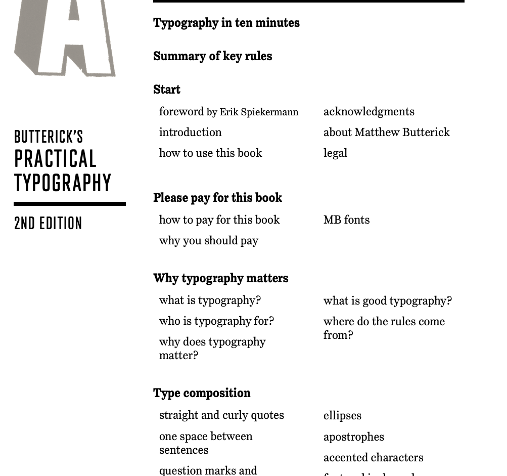
![](img/practical-typography.png)

---
# Identify fonts

Use others work to help you - I found the font for these slides from a different theme that I liked.

Use google chrome's developer tools to help!

--
Also consider downloading fonts (from google or wherever) and using them directly.

Check out this [great blog post](https://yjunechoe.github.io/posts/2021-06-24-setting-up-and-debugging-custom-fonts/) by June Choe.

---
class: inverse-red middle

# Dashboards!

---
# The definitive source!
https://rmarkdown.rstudio.com/flexdashboard/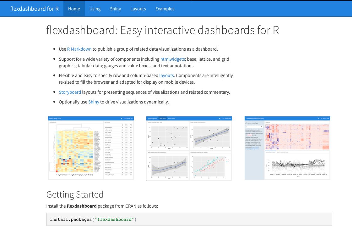

![](img/flexdashboards.png)

---
# Example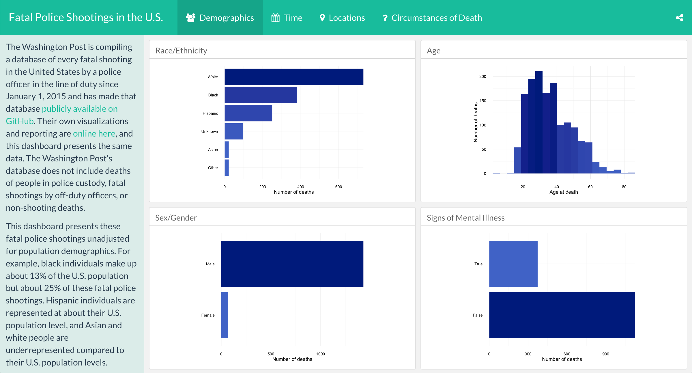

![](https://arm.rbind.io/slides/img/flexdashboard-fatalpoliceshootings.png)

.footnote[Credit: This example from [Alison Hill's rstudio::conf(2019L) class]()]

--
By [Julia Silge](https://juliasilge.com) (see the [blog post](https://juliasilge.com/blog/fatal-shootings/), [dashboard](https://beta.rstudioconnect.com/juliasilge/policeshooting/policeshooting.html),
and [source code](https://gist.github.com/juliasilge/9acbe97c549502bac85404779edceba0))

---

![](https://arm.rbind.io/slides/img/flexdashboard-mosaic.png)

.footnote[Credit: This example from [Alison Hill's rstudio::conf(2019L) class]()]

--
By [Jennifer Thompson](https://jenthompson.me) (see the [blog post](https://jenthompson.me/2018/02/09/flexdashboards-monitoring/), [dashboard](https://jenthompson.me/examples/progressdash.html),
and [source code](https://github.com/jenniferthompson/MOSAICProgress))

---
# Getting started

```r
install.packages("flexdashboard")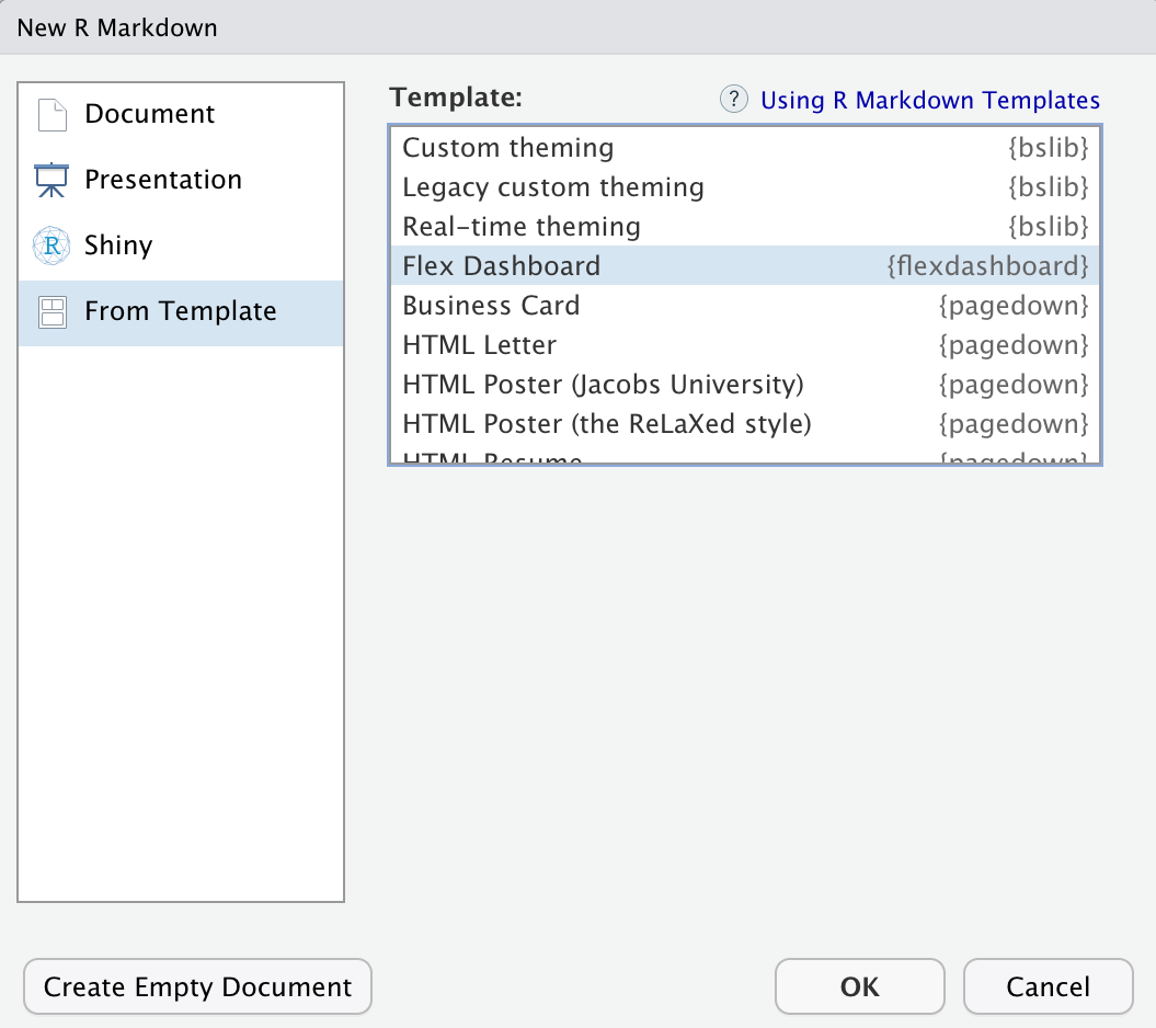
```

![](img/new-flexdashboard.png)

---
class: inverse-red middle center
# Do it
### knit right away
### Add some plots
### Play

---
# Columns

* Define new column with

```
Column
----------------------------------
```

* Optionally specify the width with `{data-width}`

--
* Annoyingly, be careful with spacing!

`{data-width=650}` will work

### but

`{data-width = 650}` will not work

---
# New squares

```md
### Square title
< r code chunk >
```

* Each time you add a square it will split the area evenly among all the squares

---
# Thinking in rows

* Change the YAML to

```md
output: 
  flexdashboard::flex_dashboard:
    orientation: rows
```

* Each `###` will then create a new column

--
* Add new rows with

```md
Row
----------------------------------
```

--
* Modify height with `{data-height=XXX}`

---
# Pages
You can easily specify multiple pages by just specifying a Level 1 Header

```md
# Page 1

Column {data-width=650}
----------------------------
### Chart A
< r code>

Column {data-width=350}
----------------------------
### Chart B
< r code>

### Chart C
< r code>

# Page 2

```

---
# A brief aside on interactivity

* Things like `reactable::reactable` and `plotly::ggplotly` can help give your dashboard some nice interactvity.

--
### However!
* If you have more than one page, you'll have to turn it into a shiny app (basically)

* This is not as hard as it sounds!

---
# Steps to interactivity
### With multipage layouts

Add `runtime: shiny` to your YAML

```
---
title: "My amazing dashboard"
runtime: shiny
output: 
  flexdashboard::flex_dashboard:
    orientation: columns
    vertical_layout: fill
---
```

--
Save your interactive piece into an object, and call the corresponding `render*` fucntion.

.pull-left[

```r
p <- ggplot(...)
renderPlotly(p)
```
]

.pull-right[

```r
tbl <- reactable(...)
renderReactable(tbl)
```
]

---
# Sidebar
* Julia Silge's had a nice sidebar where she explained things about the flexdashboard... You can have this too!

```md
Sidebar Title {.sidebar}
--------

Your text here. You can use markdown syntax, including 
[links](http://blah.com), *italics*, **bolding**, etc.   
```

--
* Multiple pages? Just change the separator to keep it there

```md
Sidebar {.sidebar}
============

Your text here. You can use markdown syntax, including [links](http://blah.com), *italics*, **bolding**, etc.   
```

---
# Tabsets

This is actually a standard R Markdown feature, but you can use it with flexdashboards as well

```md
Column {.tabset}
----------------------------------------------------------------------

### Chart 1
< r code>

### Chart 2
< r code>

### Data Table
< r code>
```

--
No comma between multiple column arguments

.pull-left[
### Good
```
Column {.tabset data-width=650}
```
]

.pull-right[
### bad
```
Column {.tabset, data-width=650}
```
]

---
# Icons
* Probably not the most important thing, but fun

* Use Font awesome!

```md
# Years {data-icon="fa-calendar"}
```

---
# HTML Widgets

Add a touch of interactivity

* Plenty of HTML widgets for R out there (see https://www.htmlwidgets.org/showcase_leaflet.html)

* {plotly} is cool

```r
library(plotly)
p <- ggplot(mpg, aes(displ, cty)) +
  geom_point() +
  geom_smooth()

*ggplotly(p)
```

---
# Including Text

* If you want to include text about an overall figure, just put the text in the R Markdown doc like you normally would

```md
# Base {data-icon="fa-calendar"}
Here's a description about the plot that follows

### A base R plot
< r code>

```

---
# What if you have tabsets?

* Works great if you want to describe all the plots/tables/content in the tabset

* If you want to provide text for an individual plot, use `>`

```md

Column {.tabset data-width=350}
-------------------

This text will describe the full tabset

###  Chart 1
< r code>

> Here's some text for Chart 1

###  Table 1
< r code>

> Here's some text for Table 1

```

---
# Storyboarding

* A little bit advanced, but pretty cool

* First, change the YAML

```md
output: 
  flexdashboard::flex_dashboard:
    storyboard: true
```

---
```md
# Method {.storyboard}

### Sample Descriptives {data-commentary-width=400}
< r code>

****

This is some text describing what's going on with the sample, and how we moved from the raw data tot he analytic sample.

### Correlation Matrix {data-commentary-width=200}
< r code>

****

There is less to say here so I made the commentary box smaller

# Results {.storyboard}

### Plot 1 {data-commentary-width=600}
< r code>

****

Lots to say here. There is important

### Plot 2 {data-commentary-width=200}

****

Move along

```

---
# Customization
* Add font-awesome stuff
* Change the [theme](https://rmarkdown.rstudio.com/flexdashboard/using.html#appearance)

```md
flexdashboard::flex_dashboard:
  theme: readable
```

---
# CSS

More on this later slides

Change the navigation bar to bright pink with thin blue border

```css
.navbar-inverse {
  background-color: #FE08A5;
  border-color: #0822FE;
}
```

---
Save the previous code in "custom.css" then specify in the YAML

```md
  flexdashboard::flex_dashboard:
    css: custom.css
```

Making sure "custom.css" is in the same directory as your flexdashboard Rmd.

---
# Add a logo and favicon

```md
output: 
  flexdashboard::flex_dashboard:
    logo: logo.png
    favicon: favicon.png
```

---
class: inverse-red middle

# Websites w/Distill

---

# Sub-agenda 
* Introduce Distill
* Deployment

--
### Learning objectives
* Get at least a basic site deployed

**By the end of the day! You will have a site!**

---
class: inverse-blue middle

# Distill
https://rstudio.github.io/distill/

---
# Please follow along

```r
install.packages("distill")

# or

remotes::install_github("rstudio/distill")
```

---
# Back to RStudio

### Create new project
<img src = "img/create-blog.png" height = "350px">

---
# The steps
* Create a new RStudio Project

* Select distill blog
  - **Make sure** to Select "Configure for GitHub Pages"

---
# Author a new article
* `distill::create_post()`

* Create another one!

---
# Build your website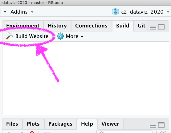
![](img/website-build.png)

---
class: inverse-blue middle
# Connect to GitHub
## Use the project-first workflow and publish the docs folder

.center[
[Demo]
]

---
class: inverse-red center middle
# That's basically it! 🎉

--
## A few additional features

---
# Categories

* You make up the category names. Tag posts with those categories, and they will be linkable

```yaml
---
categories:
  - dataviz
  - class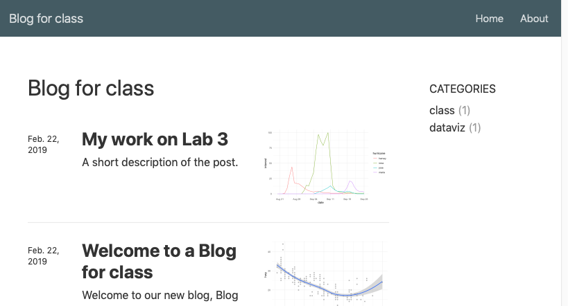
---
```

![](img/categories.png)

---
# Navigation

All controlled with `_site.yml`

* Let's add a github logo that links to our repo

--
```
---
navbar:
  right:
    - text: "Home"
      href: index.html
    - text: "About"
      href: about.html
    - icon: fa fa-github
      href: https://github.com/datalorax/class-site-example
---
```

---
# Create drop-down menus

```
---
navbar:
  left:
    - text: "Labs"
      menu:
        - text: "Getting Started with R"
          href: "lab1.html"
        - text: "Visualizing Distributions"
          href: "lab2.html"
  right:
    - text: "Home"
      href: index.html
    - text: "About"
      href: about.html
    - icon: fa fa-github
      href: https://github.com/datalorax/class-site-example
---
```

---
# Base URL
Once your site is deployed (or you know the link it will be deployed to), change the `base_url` in the `_site.yml`

* Gives some nice sharing features (twitter cards)

* Allows you to use [citations](https://rstudio.github.io/distill/citations.html)

---
# Drafts
If you want to work on a post for a while without it being included in your website, use `draft = TRUE`

`distill::create_post("My new post", draft = TRUE)`

```
---
title: "My work on Lab 3"
description: |
  This lab was hard!
draft: true
---
```

---
# Figures

Change figure options with chunk options

* `layout = "l-body"` (default)
* `layout = "l-body-outset"`
* `layout = "l-page"`
* `layout = "l-screen"`
  + `layout = "l-screen-inset"`
  + `layout = "l-screen-inset shaded"`

### Try it out!

---
# Additional figure options

* Rather than using `![]()`, you can use `knitr::include_graphics()` to have the same options.

* Use `fig.cap` in chunk options to give nice figure captions.

* Note these options should work for tables as well

---
# Side notes

```
<aside>
This is some text that will appear in the margin - similar to Tufte's style. It is often used to provide extra detail.
</aside>
```

You can also use this to show small plots

```
<aside>

ggplot(mtcars, aes(mpg)) +
  geom_histogram() +
  labs(title = "Distribution of Miles Per Gallon")

</aside>
```

---
# Customizing the theme

Use `distill::create_theme("style")`

* Creates a `style.css` file (or whatevs you want to call it in the above)

* Modify `_site.yml` to

```
output:
  distill::distill_article:
    css: style.css
```

---
* Modify small elements

```
.distill-site-nav {
  color: rgba(255, 255, 255, 0.8);
  background-color: #455a64; 
  font-size: 15px;
  font-weight: 300;
}
```

becomes

```
.distill-site-nav {
  color: rgba(255, 255, 255, 0.8);
  background-color: #FF5FDD; 
  font-size: 15px;
  font-weight: 300;
}
```

---
# This can be fun!
Just be careful not to go too far: from [Yihui](https://slides.yihui.name/2018-blogdown-rstudio-conf-Yihui-Xie.html#33)

### Debugging CSS, van Gogh (1890)
.center[
<img src="https://slides.yihui.org/images/debug-van-gogh.jpg" height="300px" />
]
---
# Equations

Use latex notation and it should "just work"

`$$` `\mu = \frac{1}{n}\sum_{i=0}^n{x_i}` `$$`

becomes

.Large[
`$$\mu = \frac{1}{n}\sum_{i=0}^n{x_i}$$`
]

---
# Other features
* Table of Contents
* Appendices
* Citations
  + Both how to cite your article and bibliographies

---
background-image:url("https://images.pexels.com/photos/346796/pexels-photo-346796.jpeg?auto=compress&cs=tinysrgb&dpr=2&h=750&w=1260")
background-size:cover
class: center
# Go forth and share your work!

---
class: inverse-red middle

# Customization
With CSS

---
# Basics of HTML

HTML code is broken up like this

```html
<body>

<h1>My First Heading</h1>
  <p>My first paragraph.</p>

</body>
```

--
When we write markdown, things like `# My header` are translated to `<h1>My header</h1>`.

---
# Common HTML tags

|Tag| What it does|
|:----|:----------|
|`<body>`| The body of the document|
|`<h1>`, `<h2>`...`<h6>`| Headers |
| `<b>`, `<u>`, `<i>` | Emphasis (bold, underline, italics)|
| `<br>` | line break|
| `<p>` | paragraph (basically text)|
| `<a>` | link |
| `<img>`| image|
| `<div>`| Generic section|

---
# Modifying these with CSS

Let's start by creating an RMarkdown document

--
Add a code chunk, but swap out `r` for `css`

--
Change the body font to Times New Roman (or whatever else you want) usings something like this

```css
body {
  font-family: "Times New Roman";
}
```

We specify the thing we want to modify (`body`), then use curly braces, then put the corresponding CSS code. Note the CSS code always follows the form `thing: modifier;`.

---
# Challenge

Play around for three minutes. See if you can do the following

* Use a different font family for Level 1 headers than the rest of the document
* Change the color of the body text or one of the headers (use `color: #hexcode`).
* Try playing with `background-color`.

---
# Using google fonts
Go to [fonts.google.com](https://fonts.google.com/)

Click on a font you're interested in. Once you decide you want it, click "Select this style".

Click the `@import` button, then copy the import code between `<style>` and `</style>`. Put this near the top of your CSS file (or chunk), then use the "CSS rules" to specifically refer to it.

---
# Example google font usage

```css
@import url('https://fonts.googleapis.com/css2?family=DotGothic16&display=swap');

h1 {
  font-family: 'DotGothic16', sans-serif;
}
```

Note - this might increase the runtime for your page, but usually not significantly.

---
# Inspecting things

I highly recommend using Google Chrome's developer tools. It allows you to hover over things and see the corresponding style. You can even modify the style there to see what changes it will make.

Let's see if we can modify the background color for our code chunks in RMarkdown.

.center[[Demo]]

---
# Creating a style sheet

If you're adding more than a few lines of style (CSS), it might be good to put it all in a single style sheet, then refer to it through the YAML.

Switch

```yaml
output: html_document
```

```yaml
output: 
  html_document:
    css: mystyle.css
```

--
### Important! The spacing *really* matters here

---
# Writing a stylesheet
I would encourage you to try other text editors for writing style sheets. SublimeText and VS Code are probably the best options.

.pull-left[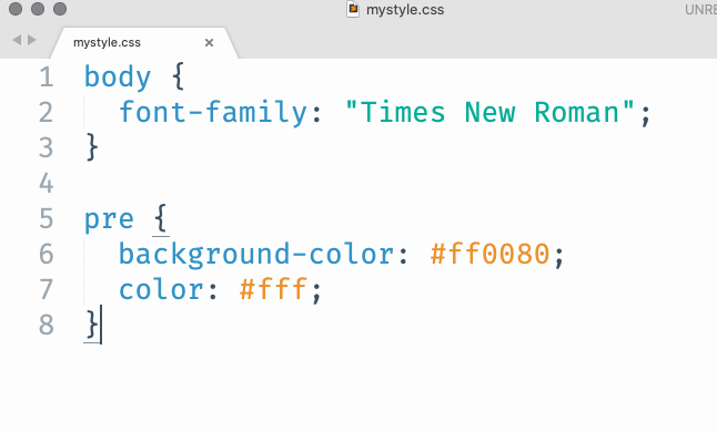
![](img/css-sublimetext.png)
]

.pull-right[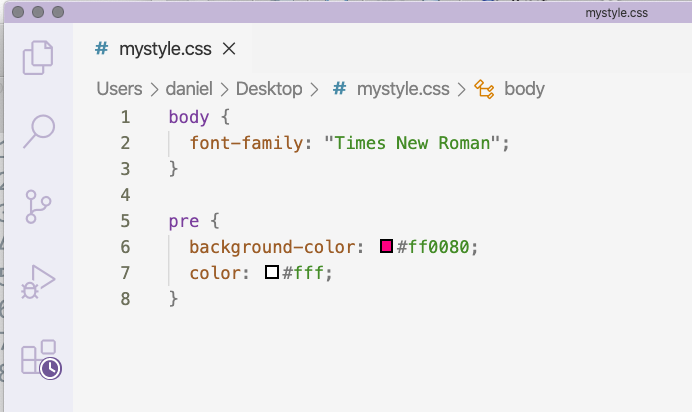
![](img/css-vscode.png)
]

There are *hundreds* of styles, but the main point is that you can get appropriate code highlighting that you can't get through RStudio (to my knowledge).

---
# Fixing our code output
This is a little complicated... because we changed our code chunks to be white (see screenshots on prior slide), the code chunk output just looks like a fully white box.

Using the inspector we can find

```css
pre:not([class]) {
  ...
}
```

Let's modify this to fix it

```css
pre:not([class]) {
  color: #ff0080;
}
```

---
# Creating new divs

You can create new divs in any RMarkdown document that uses the newest pandoc (which is most of them; some Hugo themes work better without pandoc)

```r
:::attention
Some text
:::
```

is translated to

```html
<div class = attention>
  <p>Some text</p>
</div>
```

---
# Modify your div style

Anything that has a *class* can be referred to through CSS by just adding a dot to the beginning. For example, make the text big

```css
.attention {
  font-size: 2rem;
}
```

The above says make it 2 times it's relative size.

---
# More styling for our div

Let's say we wanted to create a call-out box (i.e., to bring the reader's attention to it). We could keep modifying our `.attention` CSS code to somethign like:

```css
.attention {
  border: 3px solid #FF0380;
  border-radius: 10px;
  background-color: #ffadd6;
  font-size: 5rem;
  color: #fff;
  text-align: center;
}
```

---
# Referencing elements through their ID

Three basic ways to refer to things in CSS

```css
/*HTML tag*/
body {
  
}

/*HTML class*/
.attention {
  
}

/*HTML ID*/
#TOC {

}
```

---
# Add TOC, modify appearance

First add a TOC to your YAML

```yaml
output: 
  html_document:
    css: mystyle.css
    toc: true
```

Then add something referencing the TOC in your style sheet.

```css
#TOC {
  border: 2px solid #00FF80;
  background-color: #ccffe8;
  color: #717a75;
  border-radius: 10px;
  width: 20%;
}
```

---
# Links

Let's change the link color and hover effect. We'll do this through two different CSS chunks.

```css
a {
  color: #009954;
  font-weight: bold;
}

a:hover {
  color: #FF0380;
  text-decoration: none;
}
```

---
# A problem
In our TOC, our text doesn't stand out as much as we might want. Let's change the link style **only** for links in the TOC.

```css
#TOC a {
  color: #717a75;
}

#TOC a:hover {
  color: #FF0380;
}
```

---
# The `!important` tag

Generally best to avoid, but sometimes it's hard - using this tag will override the standard *cascading* style preference.

```css
thing {
  background-color: #ff0080 !important;
  color: #fff !important;
}
```

---
class: inverse-blue middle
# Styling flexdashboards

---
# Change the navbar color

A couple of ways to do this - modify `.container-fluid` or `.navbar`.

Let's change the navbar background color and the font. I'll add a bottom border too

```css
@import url('https://fonts.googleapis.com/css2?family=Stick&display=swap');

.container-fluid {
  background-color: #fff;
  font-family: 'Stick', sans-serif;
  border-bottom: 3px solid #00998c;
}
```

---
# Navbar title

Note - this is one area where I couldn't get it to work without the `!important` tag.

```css
.navbar-brand {
  color: #00998c !important;
  font-size: 5rem;
}
```

---
# Be gone weird other border!

The navbar has an inverse too that you might want to remove or modify

```css
.navbar-inverse {
  border: none;
}
```

---
# Overall background

```css
body {
  background-color: #001413;
}
```

---
# Chart titles

Note I've added another google font. You can do this in a single line of code with `...family=DotGothic16&family=Varela+Round&display=swap...`

```css
.chart-title {
  background-color: #fff;
  font-family: 'Varela Round', sans-serif;
  color: #00998c;
  font-size: 3rem;
}
```

---
# Panel backgrounds

```css
.chart-stage {
  background-color: #f5fffe;
}
```

---
# Style plot to match theme

```r
library(ggplot2)
library(showtext)
font_add_google("Varela Round", "vr")
showtext_auto()

ggplot(mtcars, aes(disp, mpg)) +
  geom_point(color = "#001413",
             size = 3) +
  geom_smooth(color = "#00998c",
              fill = "#001413") +
  theme(plot.background = element_rect(fill = "transparent",
                                       color = NA),
        panel.background = element_rect(fill = "transparent",
                                        color = NA),
        panel.grid = element_blank(),
        text = element_text(family = "vr",
                            size = 30,
                            color = "#00998c"),
        axis.text = element_text(color = "#00998c"))
```

You'll want to use `dev.args = list(bg="transparent")` in global knitr chunk options too.

---
class: inverse-green middle

# Next time
## Tables and Geographic data